The answer, at least for seven rivers of the Amazon Basin, seems to be negative, as we try to demonstrate in a paper that was recently published in Geology. My coauthors are Paul Durkin, at the University of Manitoba, and Jake Covault, at the Bureau of Economic Geology, The University of Texas at Austin. In this blog post, I try to provide a bit more background to our paper.
Why is this an interesting result? After all, it makes sense that there is more outer bank erosion in sharper bends. Erosion is primarily a function of the shear stress exerted on the bank; and shear stress is high where the high-velocity core of the river gets close to the bank (because in this case flow velocity has to quickly decrease from a maximum to zero, and shear stress is a function of the rate of change in velocity). The high-velocity core gets pushed close to the bank if the centrifugal force is large; and the centrifugal force is directly proportional to curvature, 1/R (where R is the radius of curvature). In short, if we use the simplest, most pedestrian physical reasoning, we would expect that erosion, and therefore bank migration, are high in high-curvature bends. However, a lot of previous work on meandering rivers suggests that this is not the case.
The Hickin and Nanson (1975) curvature-migration-rate plot
At a time when time-lapse satellite imagery was not available, Edward Hickin and Gerald Nanson (at Simon Fraser University at the time) went to the Beatton River in British Columbia and estimated the ages of the point bars along ten transects, using dendrochronology (coring trees and counting tree rings). They wrote up the results in GSA Bulletin in what has become a highly-cited, classic paper in fluvial geomorphology. It was the first time that migration rates were estimated carefully in the field and a first opportunity to explore the relationship between meander bend geometry and migration rate. For the ten bends Hickin and Nanson have examined, they have averaged the radii of curvature measured from scroll patterns that were less than 250 years old; and, to get the migration rate, calculated the growth rate of the point bars along each transect. Then they plotted migration rate against R/W (where W is channel width):
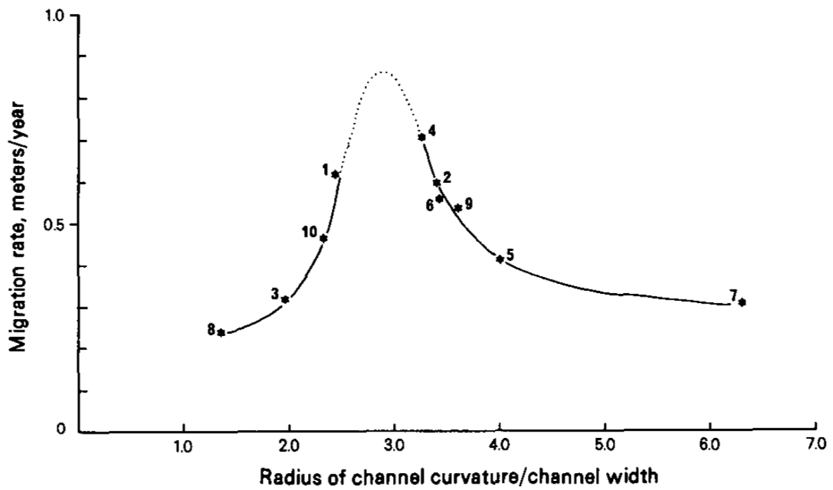
This plot suggested that migration rates are low at large values of R/W (low-curvature bends), reach a maximum at R/W ~ 3.0, then decline again with decreasing R/W (high-curvature bends). Hickin and Nanson thought that a probable explanation for this pattern could be found in the work of the famous Ralph Bagnold and Luna Leopold, work that focused on how resistance to flow varies in curved pipes and open channels. The abstract of Bagnold’s USGS report from 1960 [PDF link] sums up the key points very well:
“Resistances of pipe bends are known to fall to a sharply defined minimum when the curvature ratio, mean radius to diameter, is between 2 and 3. Recently measured flow resistances of sinuous open channels disclose that the same minimum occurs at approximately the same curvature ratio.”
Hickin and Nanson linked low erosion rates at high curvatures to high flow resistance:
“Resistance to flow rapidly increases at R/W < 2.0 because the separation zone at the concave bank breaks down and generates large turbulent eddies. The present evidence suggests that there is a corresponding reduction in the erosive work done at the concave bank.”
The separation zone they refer to (I have the impression that the first ‘concave’ in the above quote should be ‘convex’) is illustrated in one of Bagnold’s figures:
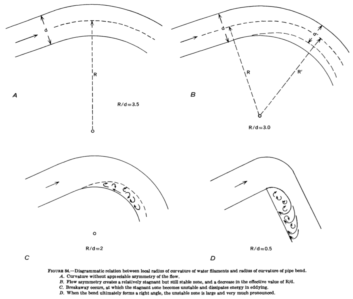
This process of within-flow energy dissipation, with reduced friction along the banks, is not very intuitive. I would expect high shear stresses and erosion rates on the downstream side of the bends shown in (C) and (D) above, as inertia pushes the high-velocity core of the flow close to the outer bank. But science is not based on intuition, and, as more and more data was collected on river migration rates, the early observations of Hickin and Nanson seemed to be largely confirmed. In the abstract of a 2011 review paper of hydrodynamic processes in sharp bends, Koen Blanckaert wrote that
“The migration rate of sharp meander bends exhibits large variance and indicates that some sharply curved bends tend to stabilize. These observations remain unexplained.”
He also summarized most of the existing data on the curvature - migration rate relationship:
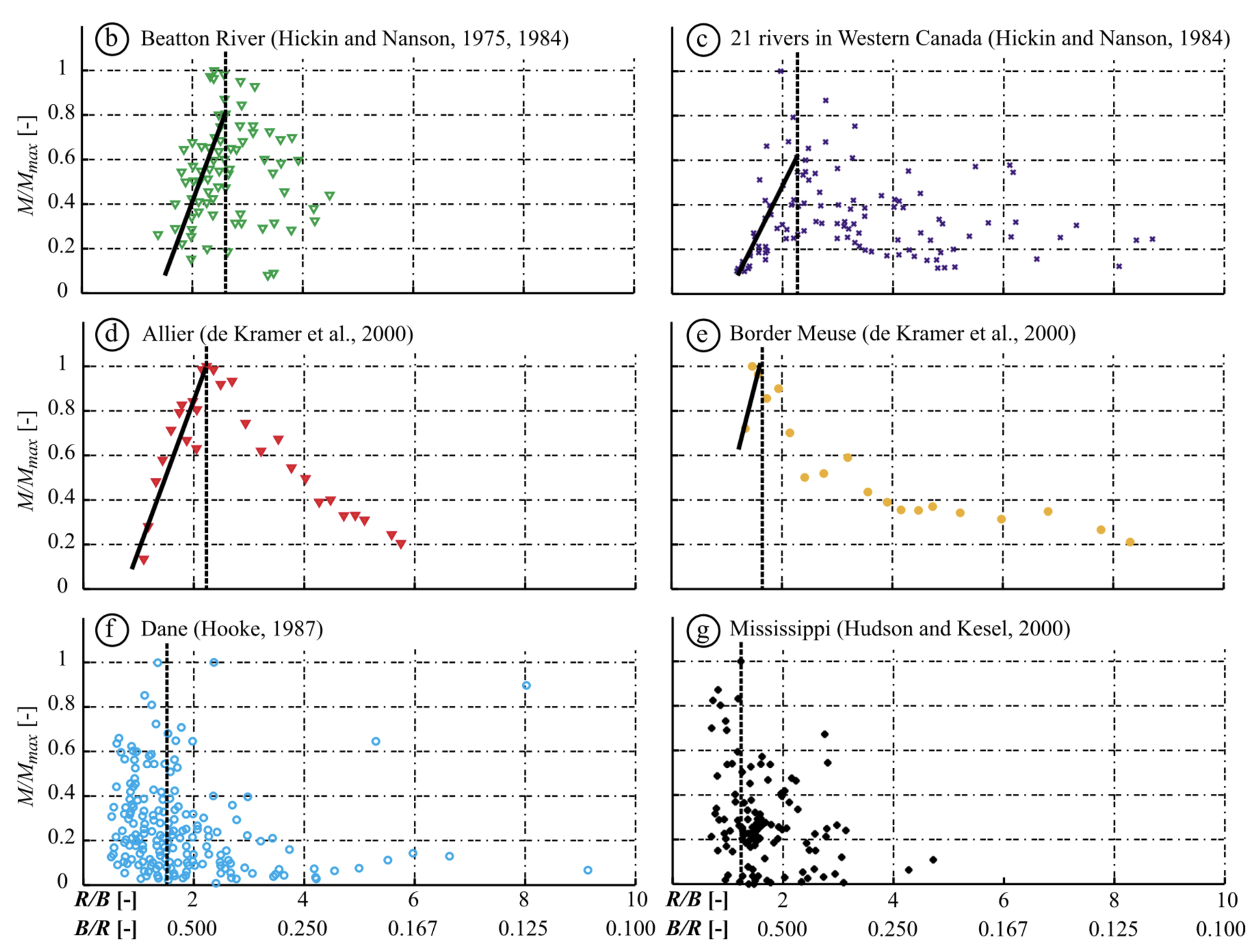
The thick black lines in the first four panels indicate the inverse relationship between migration rate and R/W in high-curvature bends. In some datasets (e.g., the lower two panels above) the scatter has increased significantly, so much so that the only obvious conclusion could be that “the migration rate of sharp meander bends exhibits large variance”; but this did not prevent the original Hickin & Nanson (1975) plot to dominate most discussions of river migration rates.
An early warning that it is not that complicated
There is an important exception: in a Geology paper published more than 30 years ago, David Jon Furbish has argued that “a single value of migration rate is not, in general, associated with a single curvature value”. A simple thought experiment suggests that this is the case. Bends with the same constant curvature can wrap around the same circle over shorter or longer distances; and it is easy to imagine that shear stresses - and therefore migration rates - in the longer bend are larger (figure from Furbish, 1988):

Think about which of these two bends would be easier to drive through (especially if the road was icy). The answer is obvious, despite the fact that the bends have the same curvature.
Furbish also showed how the maximum migration rate observed by Hickin and Nanson is likely to be an apparent maximum; and argued that a simple convolution model, that computes migration rates as the weighted sum of upstream curvatures, is a good framework to analyze the curvature - migration rate relationship. However, these arguments have largely been ignored in the fluvial geomorphology literature: the idea that high-curvature bends have low migration rates continued to persist.
So what’s new in our paper?
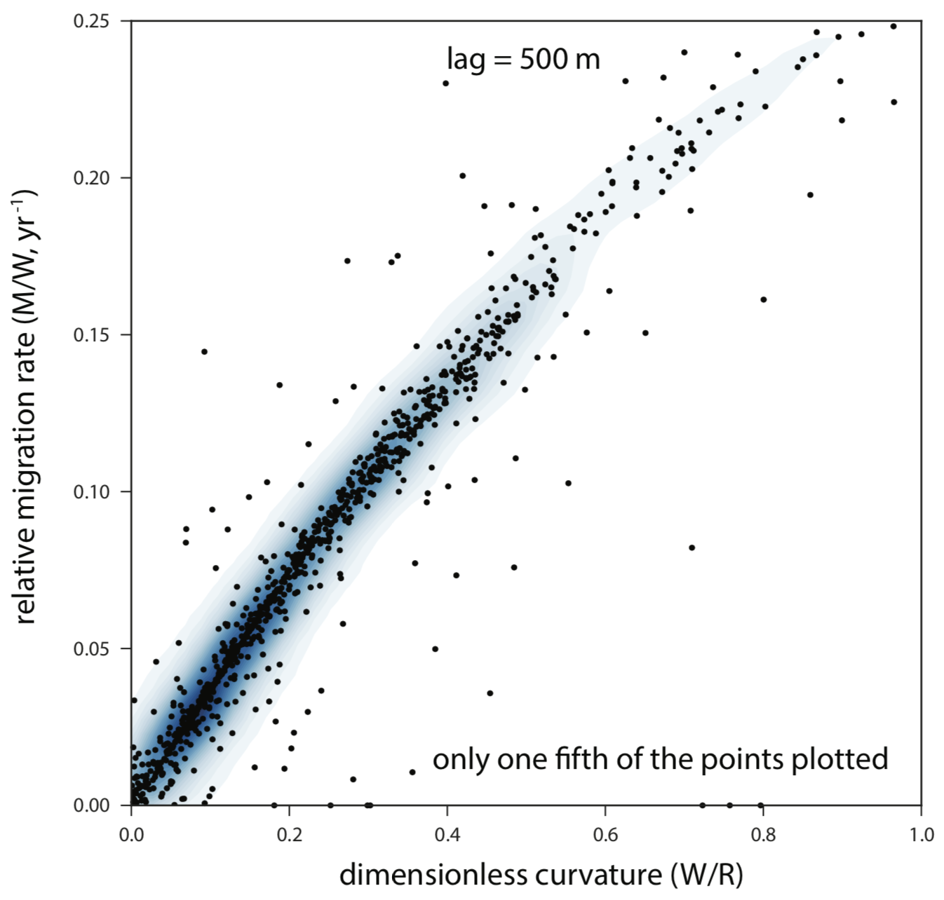
In our paper, we have reevaluated the link between curvature and migration rate, using time-lapse Landsat imagery of seven rivers in the Amazon Basin. We found that there is a strong quasi-linear relationship between curvature and migration rate. Lots of details on what exactly we did are - of course - in the paper and the supplementary file; but maybe it is worth going through some of the ideas here as well.
Measuring migration rates
A first important point is that, if we are interested in how migration rate (M) depends on curvature (1/R), and we have reasons to believe that larger curvatures cause more erosion (as I think we do), it is better to plot M as a function of 1/R or W/R, as opposed to R/W. Doing the latter would result in a hyperbola if there was a linear relationship between M and 1/R. In fact, some of the published plots look like noisy hyperbolas, e.g. (from Hudson and Kesel, 2000; red line by me):

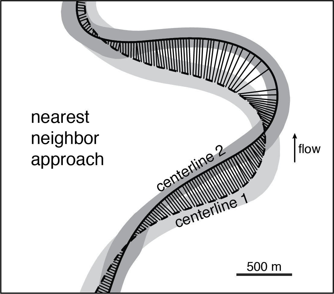
Second, it is possible to measure local migration rates as opposed to averages over entire bends. This approach eliminates the need to subdivide the channel into bends; and it has the potential of improving the signal-to-noise ratio, as both curvature and migration rate vary a lot within every bend. Given two channel centerlines that come from the same channel but represent different times and are defined by a number of points, the task is to link those points in a way that approximates the migration of the channel. One possibility is to use a nearest-neighbor approach, which links every point on the first centerline to the nearest point on the second centerline:
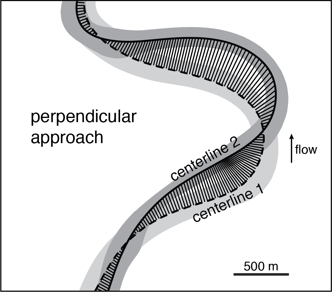
This is a start, but it would be nice if (1) the migration vectors were roughly perpendicular to the first centerline (after all, that is how erosion / accretion rates are measured, and that is the assumption in models of meandering); and (2) there were no major gaps between the correlated points on the second centerline. Let’s see what happens if we draw segments that are perpendicular to the first centerline:
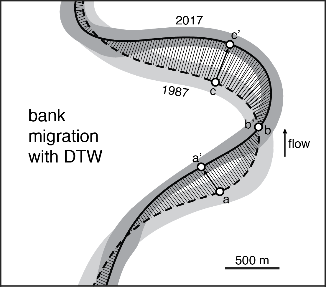
This is clearly a better result; however, it requires the definition of new points with variable spacing on the second centerline. Computationally this is quite complicated and expensive. It would be nice if it was possible to only use the existing centerline points yet get a solution that approximates the perpendicular approach shown above. It turns out that the dynamic time warping (DTW) algorithm does exactly that. With this algorithm, every point on the first centerline gets an equivalent point on the second centerline; and vice versa. In addition, it minimizes the divergence of migration vectors:
We have used a Python implementation of dynamic time warping, the dp_python package (written by Dan Ellis). I have experimented with other implementations of DTW as well (e.g., dtwalign, but found that dp_python gave the best results.
Bank migration vs. bend migration
During the review process, one of the most debated aspects of the study was whether this is the right way to measure migration rates. In bends that show significant downstream translation (like the one above), the point where the two centerlines intersect (labeled ‘b’ in the figure) does not move so its migration rate is zero. An alternative view is that the whole bend migating downstream, so maybe it is better to link points of similar curvature:
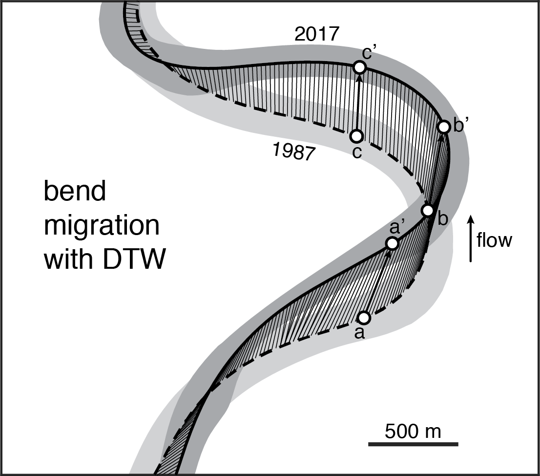
In this view, which we called bend migration, point b travels to point b’, and the migration rate is significant. This may seem like the more appropriate measure of migration, as we often talk about bend translation; and, strictly speaking, the location of point b does change a bit, depending on what second centerline you use. However, bend translation is an emergent phenomenon and is not a proxy for erosion and deposition along the channel banks. It is easier to realize this if we look at plots of erosion and deposition along the left and right banks:
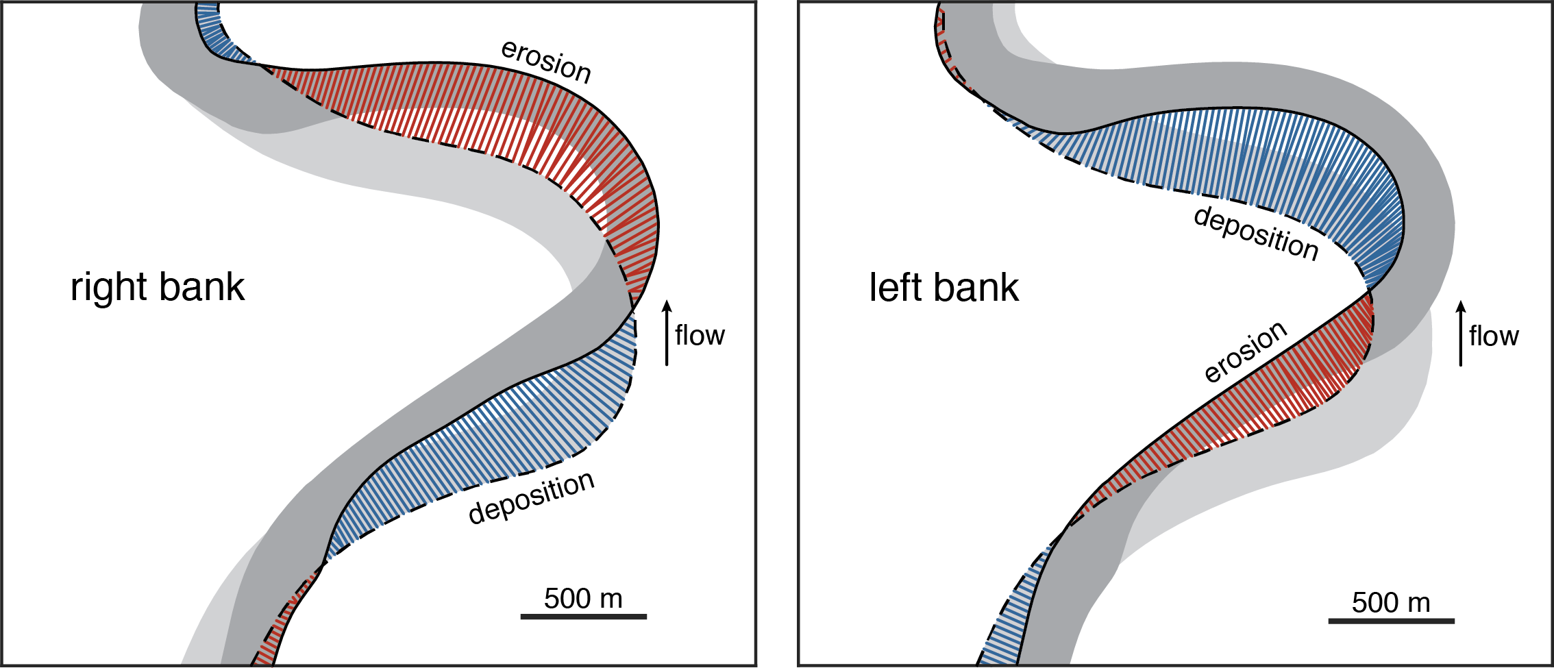
If we are primarily interested in rates of erosion and accretion along the banks (and we are), it is more appropriate to use estimates of ‘bank migration’. The bank migration rate measured on centerlines is the average of the left and right bank migration rates.
Mapping rivers
Now we know how to measure migration rates; but we need to map some rivers to perform the measurements. This can of course be done manually, but it is extremely time consuming to do that with reasonable precision. There are a number of tools now available for quasi-automatically mapping rivers in satellite imagery; we ended up using Rivamap. This Python package was developed by Leo Isikdogan, Alan Bovik, and Paola Passalacqua at UT Austin and it is based on extracting curvilinear features in an image using a so-called ‘singularity index’. We did some Python scripting to get river banks and centerlines as polygons; a bit of manual cleanup of the intermediate images was required to do this, but the speedup compared to an all-manual interpretation was still substantial.
With some manual QC and cleanup in Photoshop, the Rivamap package gets us some high-quality channel centerlines, but they are just labeled pixels in an image that need to be ordered according to their position along the centerline. The result of this process, if we zoom in to see the pixel-level detail of the MNDWI (modified normalized difference water index) image derived from Landsat data, looks like this:
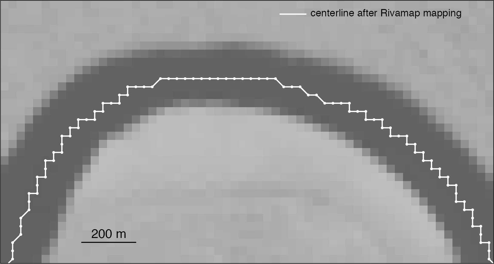
It would be of course be pointless to calculate curvature on jagged centerlines like the one above. Significant smoothing is needed, and we do that in two steps. First, we apply a Savitzky-Golay filter; this eliminates the zig-zags of the pixels:
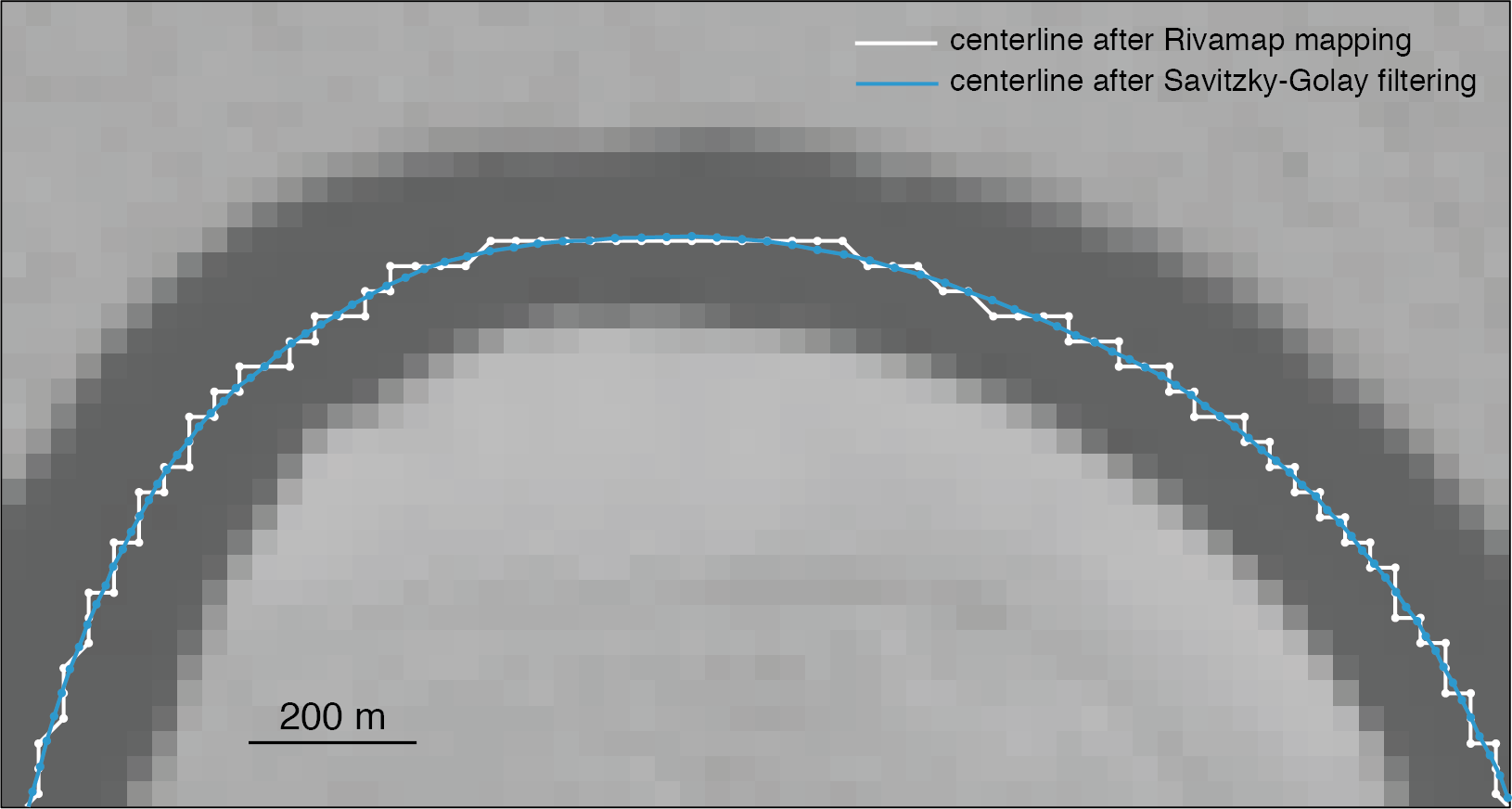
The second step is needed to get rid of the ’extra’ waviness that results in a noisy curvature series; and we do this with b-spline interpolation:

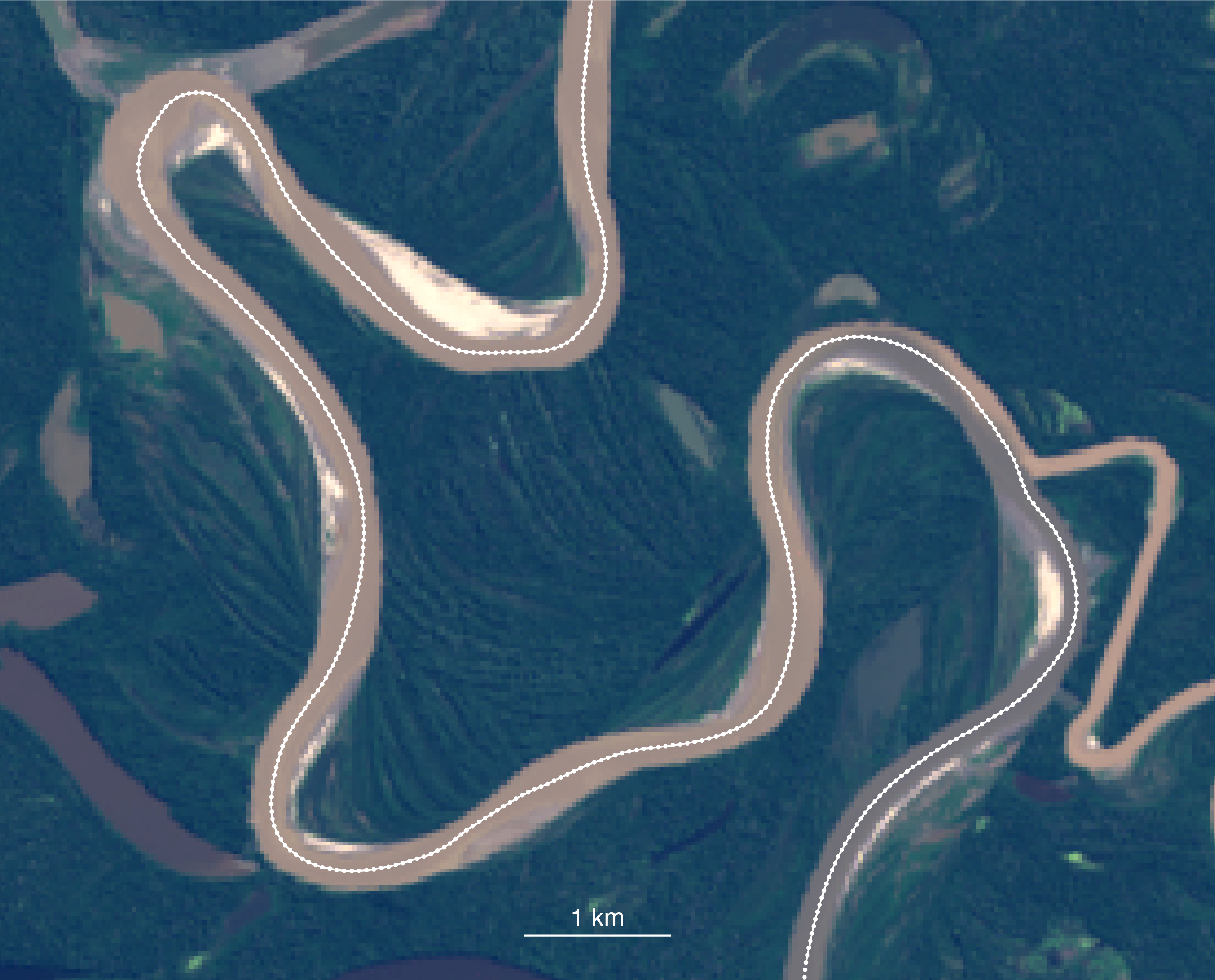
We are also interested in mapping the channel banks (although they are not necessary for measuring curvature and migration rate of the centerline). We can do that by using the centerline and the MNDWI image; to keep everything (and especially bookkeeping) simple, we discretize the banks so that every point on the centerline has corresponding points on the two banks. Here is an example Landsat image with the centerline:
And here are the corresponding banks and locations where channel widths are measured (in red):
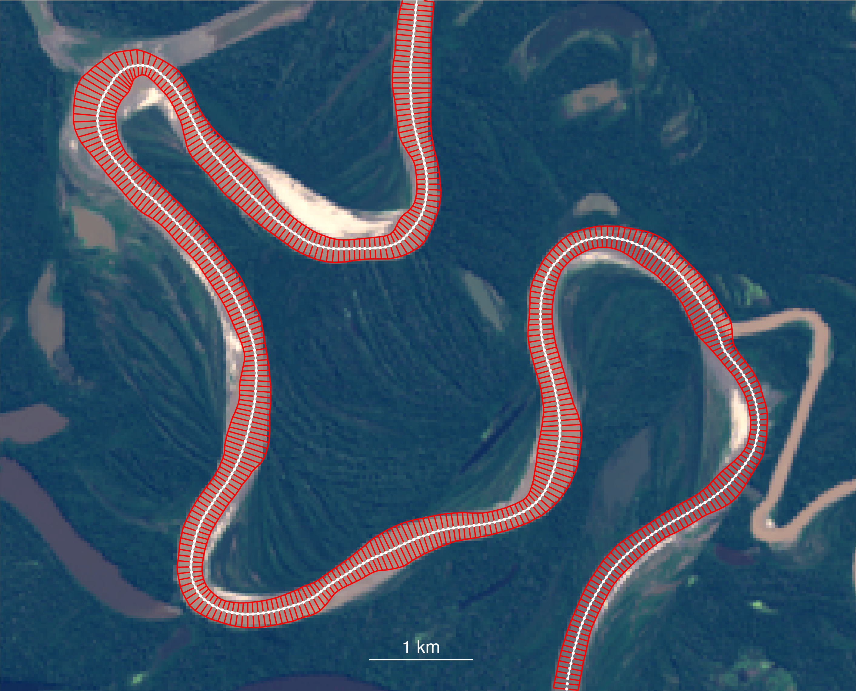
Using this workflow, a large amount of channel geometry data can be extracted relatively quickly from satellite images, with a precision close to half the pixel size (which is 30 m in the case of older Landsat data).
So we know how to map rivers and how to estimate migration rates, we can start looking at the curvature - migration rate relationship. But before we do that, I think it is useful to take a detour and think in a bit more detail about how, at least in theory, local migration rate is expected to depend on channel curvature.
The convolution model of meandering
As I mentioned before, Furbish (1988) has suggested that a simple convolution model, where migration rate is the weighted sum of upstream curvatures, is useful for understanding the dependence of migration rate on curvature. The most accessible description of a model like this can be found in a paper by Alan Howard and Thomas Knutson (1984). The key idea is that migration rate is not only a function of local curvature, but it depends on upstream curvatures as well, although the influence declines as you move upstream from the point of interest. This might seem at first sight as an arbitrary rule, but it has a strong physical basis: the same conclusion is reached if migration rate (or bank erosion) is considered as a linear function of the near-bank excess velocity, which can be computed using the shallow water equations in a curved channel. This forms the basis of another classic paper on the subject: “Bend theory of river meanders. Part 1. Linear development”, by Syunsuke Ikeda, Gary Parker, and Kenji Sawai (1981).
The convolution model of Howard and Knutson (1984) uses the concept of ’nominal migration’, the migration that would be observed if it was only a function of local curvature:
$$ R_0[i] = f(C[i]), (1)$$
where $R_0[i]$ is the nominal migration rate at location $i$ and $C[i]$ is the curvature at the same location. The simplest relationship is a linear dependence:
$$ R_0[i] = k_lWC[i], (2)$$
where $k_l$ is a constant that has the dimensions of a migration rate and W is channel width ($WC[i]$ is the dimensionless curvature). However, Howard and Knutson wanted to make sure that the curvature-migration rate relationship exhibited by the model is similar to the observations of Hickin and Nanson (which were the only data available at that time). Therefore, they used a nonlinear function for $f$ in equation (1), one that mimicks the shape of the Hickin and Nanson curve (‘Nominal Rate, Case 2’ in the plot):
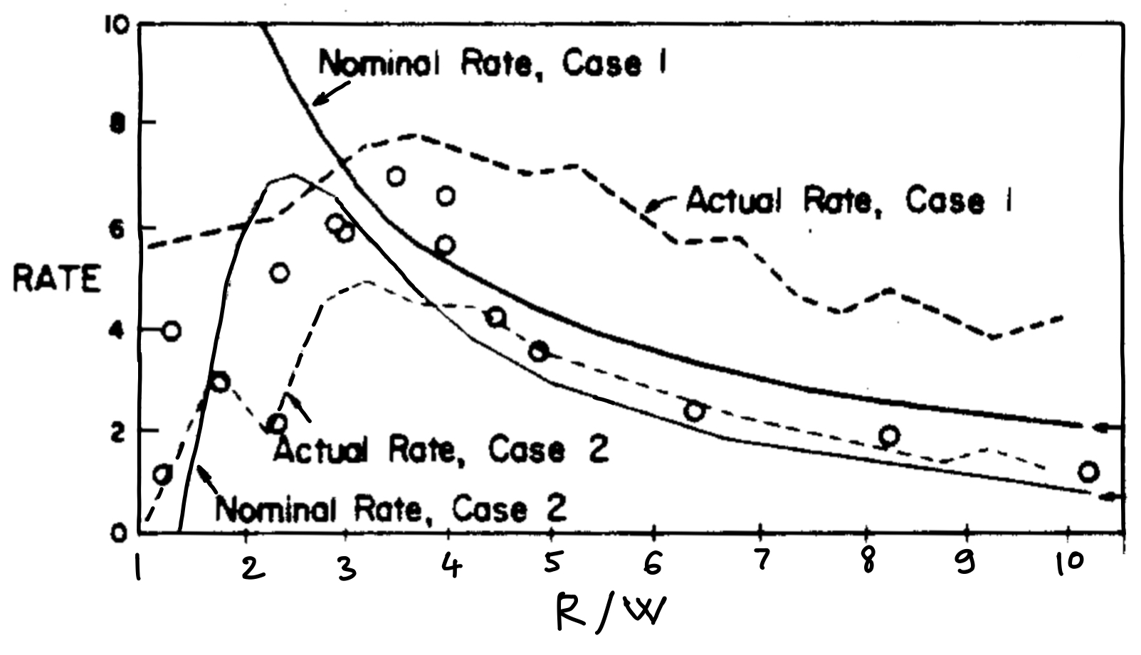
They also had a hunch that this might not be necessary and a function that allows the nominal migration rate to increase indefinitely with decreasing $R/W$ might also work (‘Nominal Rate, Case 1’ in the plot). In our implementation of the model, following the footsteps of Furbish (1988), we opted for this kind of relationship, and used equation (2) (which plots as a hyperbola on a plot of migration rate against $R/W$).
Now we can write the convolution equation for the ‘actual’ migration $R1$:
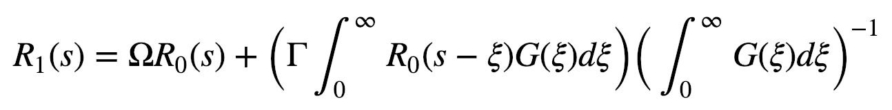
This looks more complicated than it actually is. $\Omega$ and $\Gamma$ are constants that equal -1 and 2.5; $\xi$ is the distance upstream from the point of interest, and $G(\xi)$ is a weighting function that decreases exponentially in the upstream direction:
$$ G(\xi) = e^{-\alpha\xi} $$
We call $R_1$ the ‘predicted migration rate’ (as opposed to ‘actual’), so that it is not confused with the migration rate measured in field examples. Let’s see what happens if we apply this equation to a curved channel segment that includes a couple of bends, like this one:
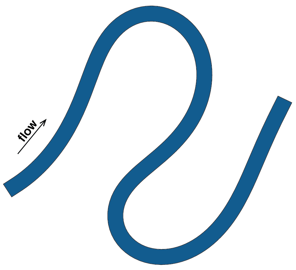
The following plot shows the nominal migration rate in blue and the predicted migration rate in red, for the channel segment above (click to enlarge):
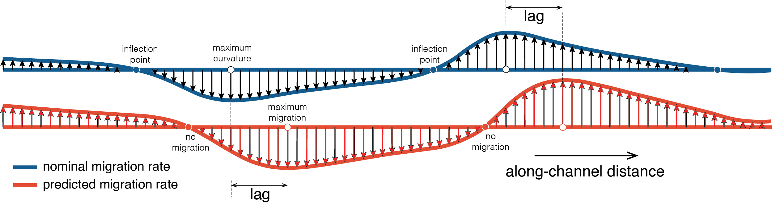
The predicted migration rate curve looks extremely similar to the nominal migration rate curve, but it is shifted downstream and the maximum values are slightly larger. The phase lag between the curves seems to be roughly constant along these bends. This downstream shift makes sense if we consider that the sum of upstream curvatures reaches a maximum value downstream from the location of maximum curvature (or nominal migration rate), where all the large curvature values of the current bend have an influence. Although the idea that the location of maximum erosion does not coincide with the bend apex has been known for a while, there is limited work on how large this phase lag is in models and in actual rivers.
This plot is also useful to think about the best approach to link measured migration rates to curvature. If you ignore the phase lag, you can see in the plot that some points of large curvature will show relatively low migration rates. This is the reason why many previous studies have found low (or variable) migration rates at high curvatures. If the phase lag is taken into account, there should be a much simpler, quasi-linear relationship. Here is the plot of predicted migration rate as a function of nominal rate for the example above, *without* considering the phase lag:
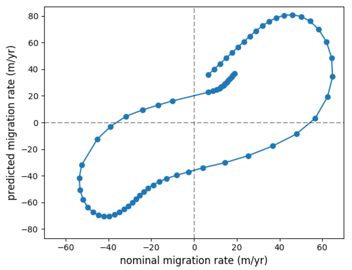
It looks like the predicted migration rate reaches maximum values for absolute values of the nominal rate of about 40 m/yr, and rapidly declines for absolute values larger than that. However, if the phase lag is accounted for, e.g., by pairing the predicted migration rate series with nominal rate values that are six positions away in the upstream dierction, we get a plot that is a lot simpler:
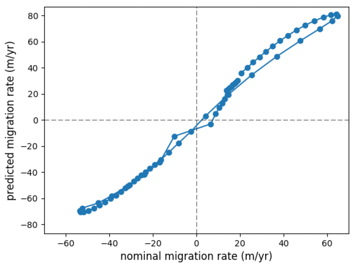
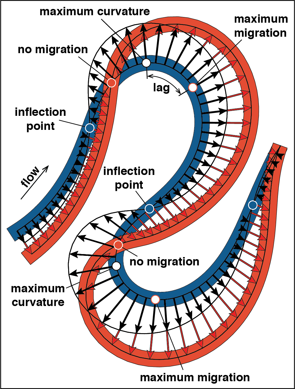
This looks like a quasi-linear relationship and the largest predicted migration rates correspond to the largest curvatures. Probably it is helpful to plot the migration rate vectors and the resulting new channel configuration in map view as well:
And here is an animation that goes through the key steps of the analysis:
The amount of migration shown here is unrealistically high, in order to illustrate the concept. The same model, of course, can be run using much longer channel segments and many more time steps. Here is an example output of a long-term channel evolution that includes numerous cutoffs and oxbow fills (shown in brown; click to enlarge):
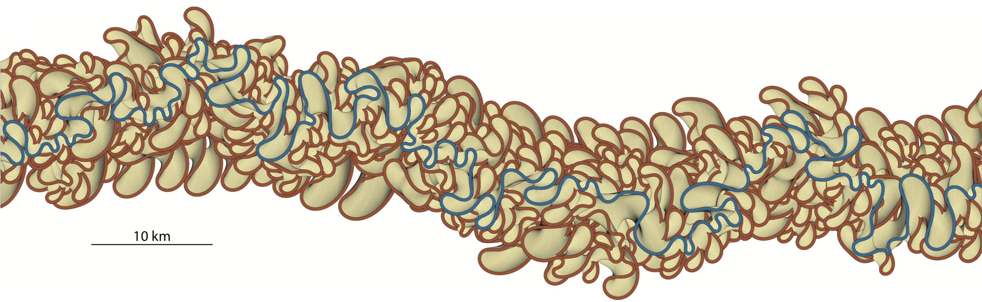
I think this is a reasonably realistic model of long-term meandering; however, there are too many teardrop-shaped, elongated bends that are not that common in nature. More sophisticated models of meandering do a better job at matching meander shapes. I think one of the interesting questions is whether they also reproduce well (or better) the migration rates and the resulting patterns. Coming back to the model above: plotting the nominal and predicted migration rates for the most recent channel, side-by-side, shows the similarity of the two curves are and the stable phase lag between the two (click to enlarge):
A plot of migration rate against $R/W$ gives a familiar shape, with an apparent maximum at $R/W$ values of about 2.5-3.0:

But we know by now that this scatterplot can be simplified if the lag between curvature and migration rate is accounted for; keeping the same axes, we get a nice hyperbola:
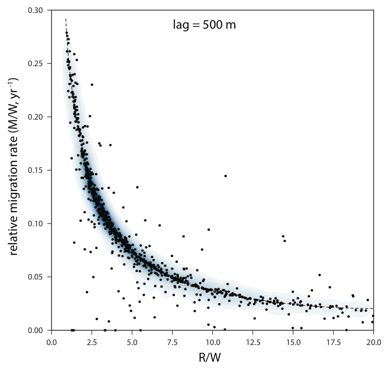
Switching to dimensionless curvature ($W/R$) on the x-axis results in a simple quasi-linear relationship:
I think these examples help to understand how the convolution model can be used to analyze the curvature - migration rate relationship. However, the question remains:
Does this work in the real world?
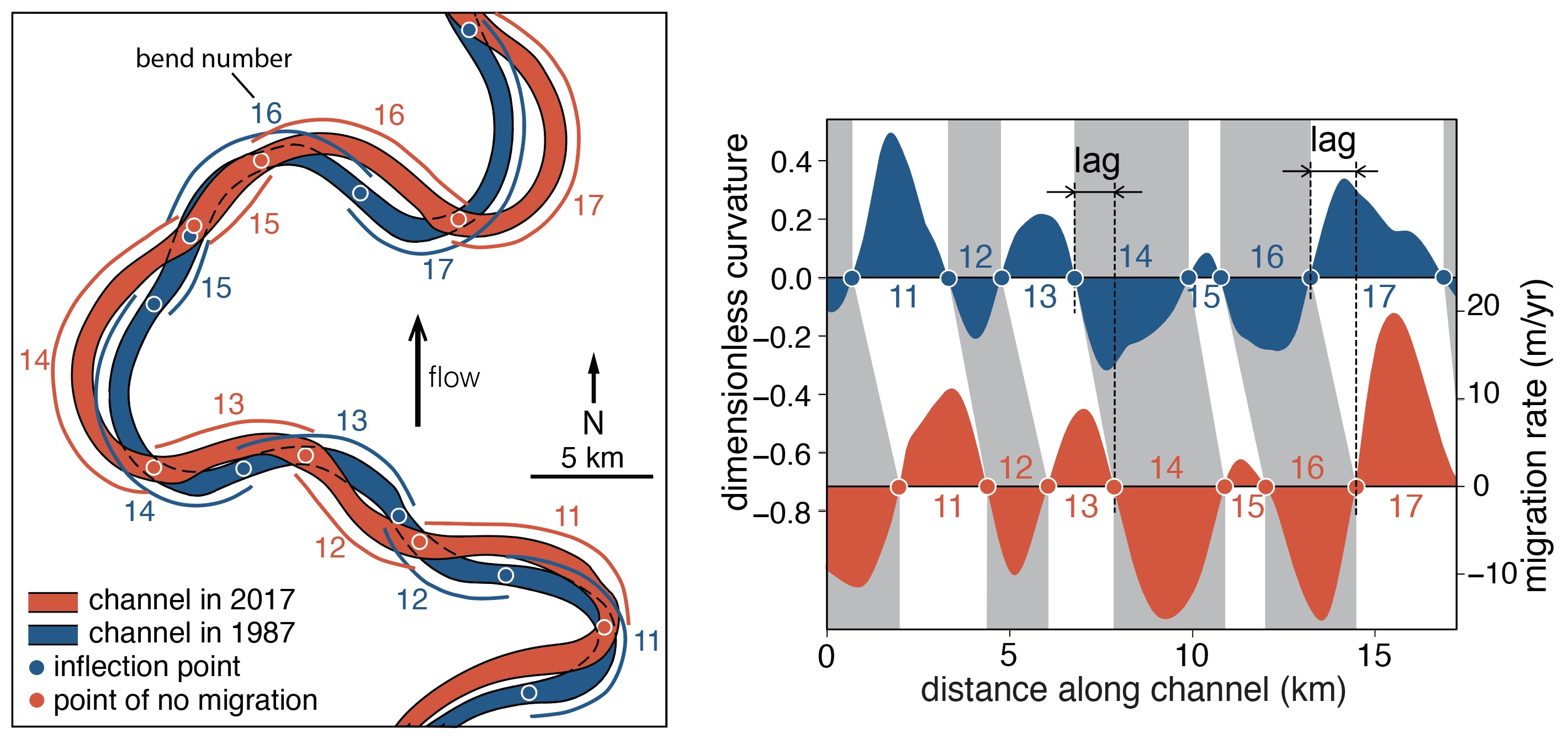
Yes, it (kind of) does. That is probably the most important result of our study. We have looked at more than 1600 bends of seven rivers from the Amazon Basin and have found that there is a remarakbly simple and strong relationship between curvature and migration rate. Here is an example showing the changes along seven bends of the Jurua River, from 1987 (blue) to 2017 (red):
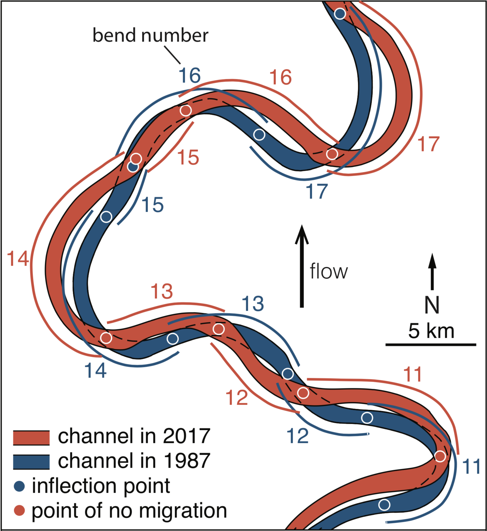
The effect of curvatures along bends defined by inflection points on the 1987 channel is felt along segments defined by the points of zero migration along the 2017 channel. This is more obvious in the plot of the curvature and migration rate series for the same bends:
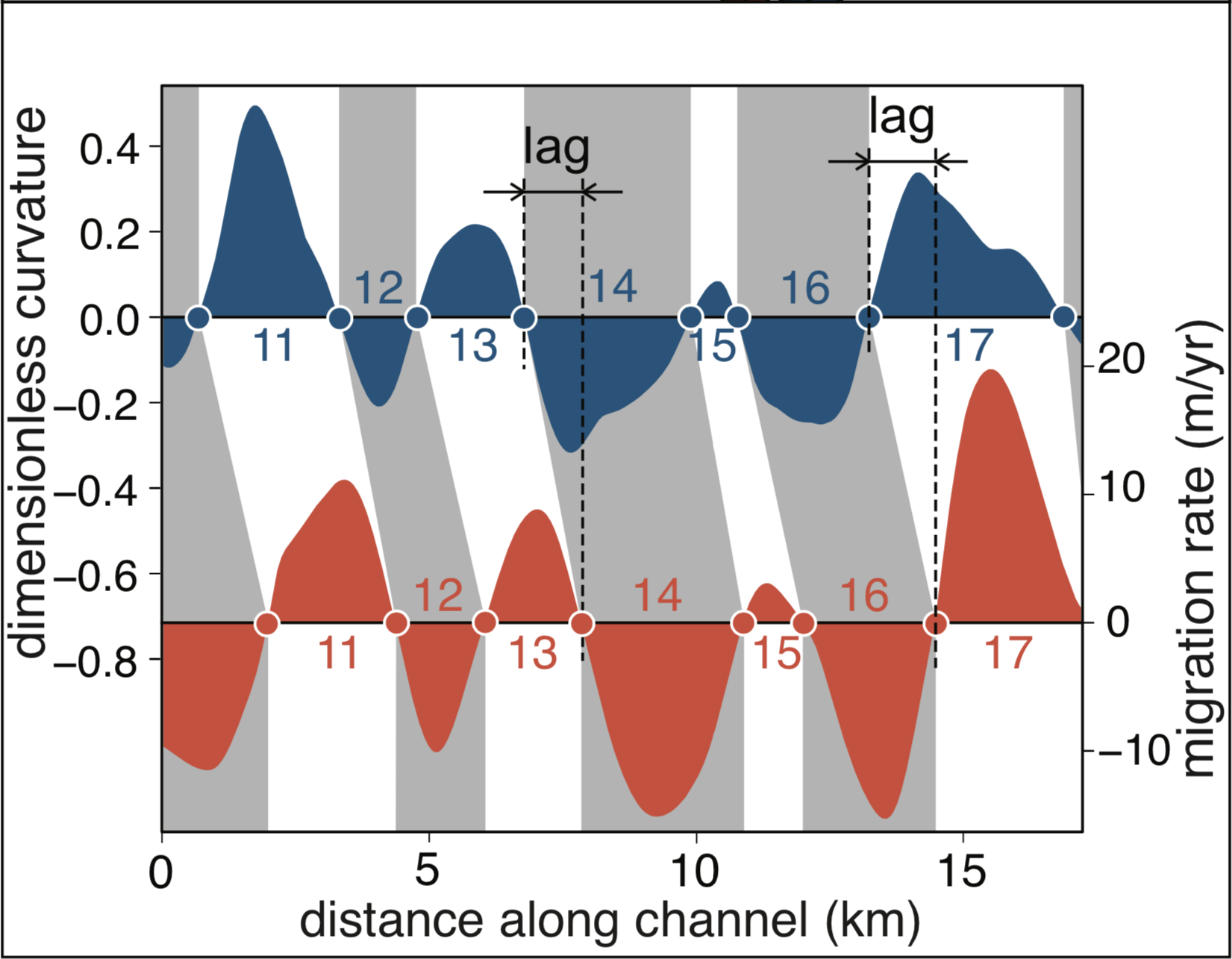
It is tempting to track the migration of bends defined by inflection points, and that is what has been done before, but the river does not care about where one bend ends and the next one starts.
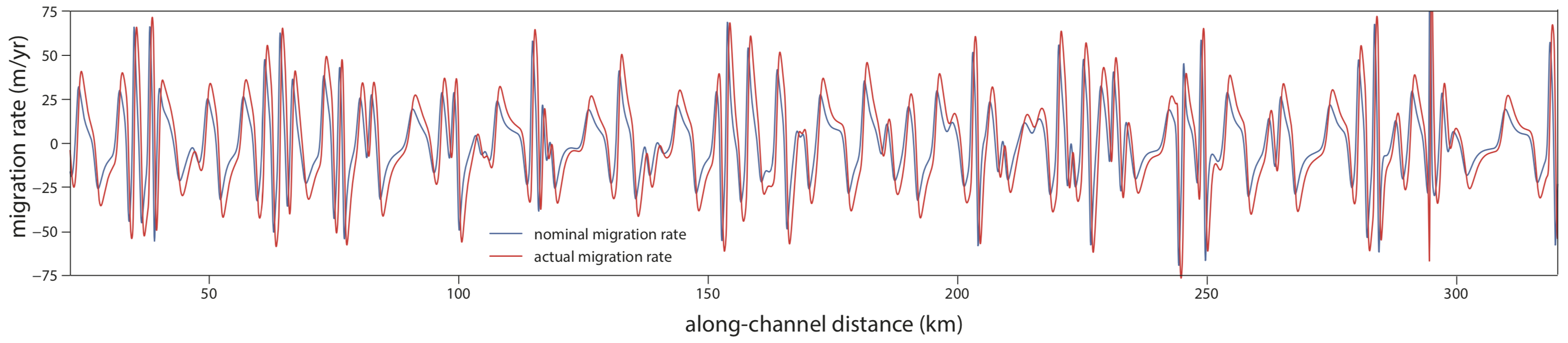
Now you might say that these seven bends were cherrypicked - and you would be right to some degree. But check out the same kind of plot for 94 bends along a 385 km long segment of the Purus River (blue = curvature, green = migration rate):
I think it is remarkable that the two curves have been measured independently yet they are quite similar to each other. This similarity is obvious if we look at the two variables in a scatterplot - with the phase lag taken into account:

The actual migration rate tends to be overall larger than the nominal migration rate, as expected from the convolution model. We can also plot the actual (measured) and predicted migration rates against each other:
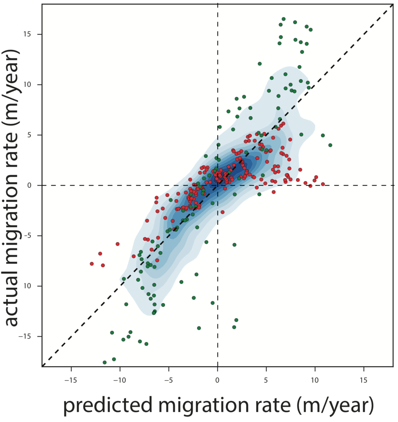
The correlation coefficient between the actual and predicted migration rates for this river segment is 0.84. In other words, more than 70% of the variance in the migration rates is explained by curvature. This illustrates the potential predictive power of our approach, at least for ‘well-behaved’ rivers.
The red dots in the plot above correspond to bends that are clearly affected by low bank erodibility (= high resistance to erosion); and therefore they show less migration than expected. We have identified these bends through looking at SRTM elevation data, in combination with the true-color Landsat images. The channel segments with resistant banks correspond to places where the river touches the erosional edges of its valley and the banks are taller and consist of older and therefore more resistant material. For example, here is an elevation map of a few bends along the Purus River:
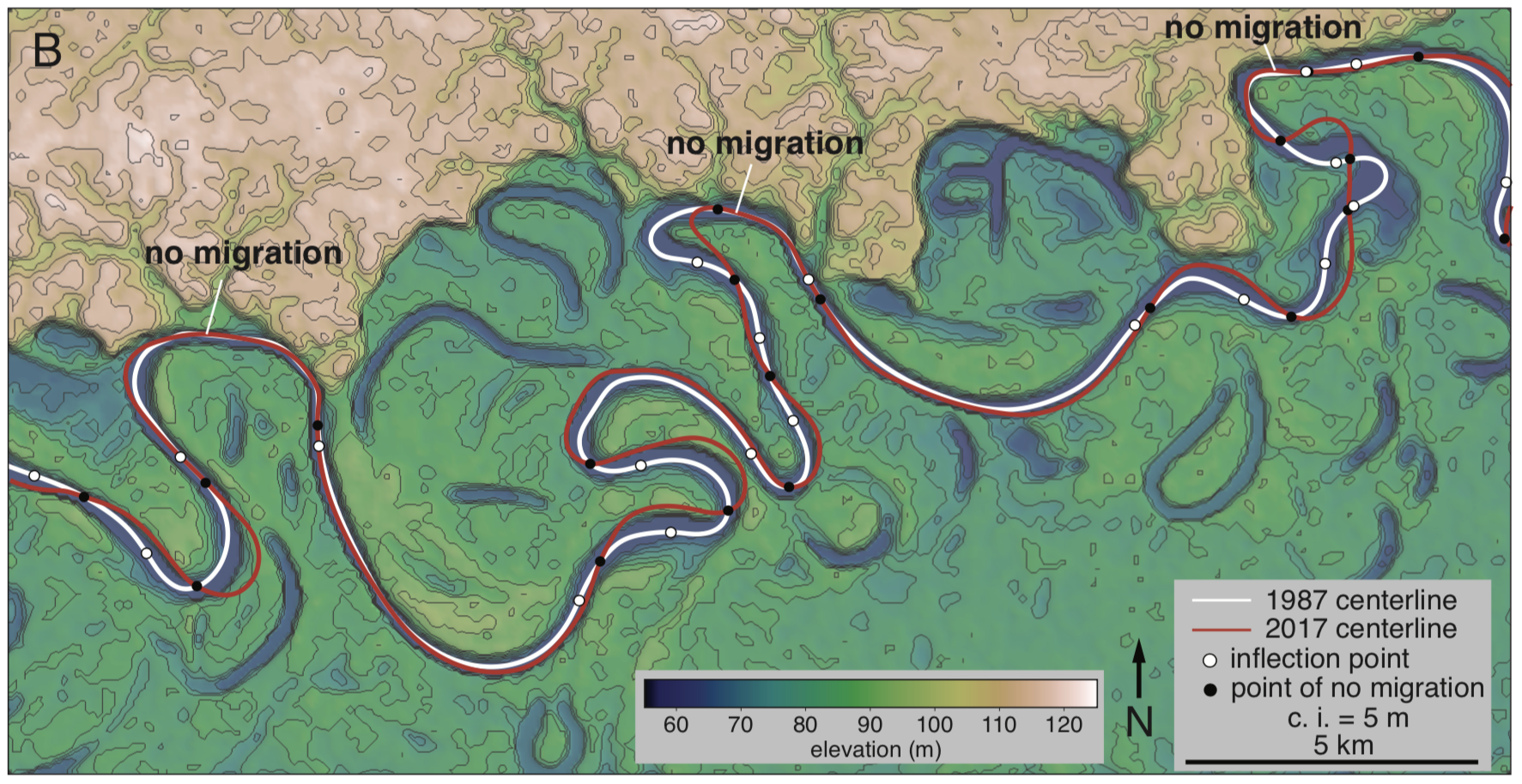
The three bends that impinge on the erosional escarpment show no migration between 1987 and 2017, while there is significant change elsewhere along the river.
The green dots come from bends that seem to be located downstream from the locations of recent cutoffs. Overall, these bends tend to have high curvatures and migrate even faster than what the convolution model predicts.
Here is an animation that goes through the steps of calculating migration rates at two points and then predicting where the channel is supposed to be after a few years:
And a longer segment of the Jurua River, showing the predicted the actual locations of the channel:
The prediction is not perfect; the model is underpredicting migration for the two bends at the top of the image, potentially as a result of the recent cutoff. Also, there is a stretch along the upper part of the first bend that does not get eroded much - my guess is that the bank is more resistant to erosion along that stretch. It is quite likely that such departures from the ‘baseline’ are so common along some rivers that the simple model that we have used becomes significantly less useful - but knowing when and where that is the case is useful in itself.
And that’s it. This post has become a bit longer than I expected, but hopefully it is a useful addendum to our paper. Here is a full list of resources related to the study:
- Geology paper
- Supplemental file
- Jackson School of Geosciences (UT Austin) press release
- Data and code on Github
- Animation of convolution model concept
- Animation of workflow for predicting migration rate in a bend
- Animation of prediction of migration rate over a few bends of the Jurua River
- Google Earth Engine apps with centerlines and Landsat images used to map them
References
Blanckaert, K., 2011, Hydrodynamic processes in sharp meander bends and their morphological implications: Processes in sharp meander bends: Journal of Geophysical Research: Earth Surface, v. 116, F01003, doi:10.1029/2010JF001806.
Furbish, D.J., 1988, River-bend curvature and migration: How are they related? Geology, v. 16, p. 752-756.
Hickin, E., and Nanson, G., 1975, The Character of channel migration on the Beatton River, Northeast British Columbia, Canada: Geological Society of America Bulletin, v. 86, p. 487-494.
Howard, A.D., and Knutson, T., 1984, Sufficient Conditions for River Meandering: A Simulation Approach: Water Resources Research, v. 20, p. 1659–1667.
Ikeda, S., Parker, G., and Sawai, K., 1981, Bend theory of river meanders. Part 1. Linear development: Journal of Fluid Mechanics, v. 112, p. 363–377, doi:10.1017/S0022112081000451.
Isikdogan, F., Bovik, A., and Passalacqua, P., 2017, RivaMap: An automated river analysis and mapping engine: Remote Sensing of Environment, v. 202, p. 1–10, doi:10.1016/j.rse.2017.03.044.